Image aesthetics quantification with a convolutional neural network (CNN)

Project report for training a MobileNetV1 based convolutional neural network (CNN) with only 14,000 images with transfer learning

Photo by Jakob Owens on Unsplash

I. Definition

Project Overview

The “A picture is worth a thousand words” stresses how important images are in the modern world. The quality of images, e.g. influences our decisions in different domains. Especially in eCommerce, where we cannot touch things they are essential. They have therefore a significant influence on our product purchasing decisions.

Which room to book?

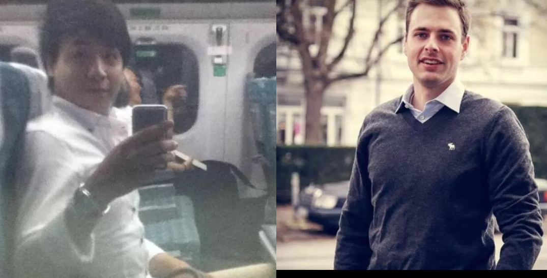Which guy to date?

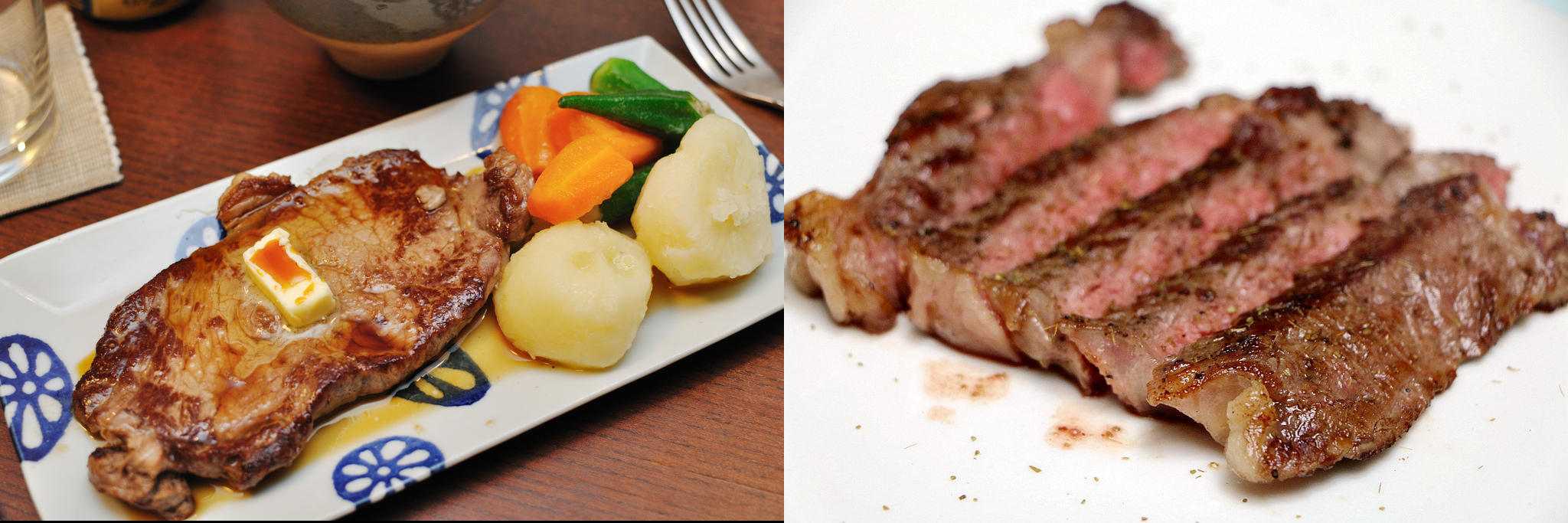Which food to order?

The goal of this project is to create a model that can quantify the aesthetics of images.

Problem Statement

The quantification of image quality is an old problem in computer vision. There are objective and subjective methods to assess image quality. With objective methods, different algorithms quantify the distortions and degradations in an image. Subjective methods are based on human perception. The methods often don’t correlate with each other. Objective methods involve traditional rule-based programming, Subjective methods are not solvable this way.

The goal of this project is to develop a subjective method of image quality assessment. As mentioned before this problem cannot be solved with classical programming. However, it seems that supervised machine learning is a perfect candidate for solving the problem as this approach learns from examples and it is a way to quantify the ineffable. A dataset with image quality annotations is a requirement for learning from samples.

Within the machine learning ecosystem, Convolutional Neural Networks (CNN) are a category of Neural Networks that have proven very effective in areas such as image recognition and classification. They are inspired by biological processes in that the connectivity pattern between neurons resembles the organisation of the human visual cortex.

The subjective quality model is implemented with a Convolutional Neural Network as it seems an excellent fit to tackle the problem.

These steps are needed:

1. Find a dataset with images with quality annotations
2. Exploratory Data Analysis (EDA) on the dataset, to evaluate the characteristics and suitability for the problem space
3. Cleanup and preprocessing of the dataset
4. Design architecture for the CNN
5. Training of the CNN
6. Test the model against benchmarks
7. Analysis of the results

There were several iterations for the steps 4.-7.

Metrics

The distribution of user ratings is predicted in the project. From there you can predict both a quantitative mean rating, but also a qualitative rating bucket. To capture these two metrics are used.

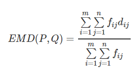
Earth Mover’s distance (EMD)

The Earth Mover’s Distance (EMD) is a method to evaluate dissimilarity between two multi-dimensional distributions in some feature space where a distance measure between single features, which we call the ground distance is given. The EMD ‘lifts’ this distance from individual features to full distributions. It’s assumed that a well performing CNN should predict class distributions such that classes closer to the ground truth class should have higher predicted probabilities than classes that are further away. For the image quality ratings, the scores 4, 5, and 6 are more related than 1, 5, and 10, i.e. the goal is to punish a prediction of 4 more if the actual score is 10 then when the real score is 5. The EMD is defined as the minimum cost to transport the mass of one distribution (histogram) to the other. (Hou, Yu, and Samaras 2016)(Rubner, Tomasi, and Guibas 2000)(Talebi and Milanfar 2018)

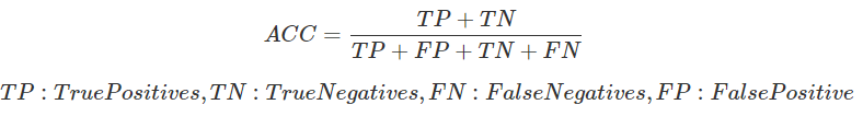
Accuracy

To compare qualitative results the Accuracy is used. The accuracy is the ratio of correct predictions. In this case, the ground-truth and predicted mean scores using a threshold of 5 on the “official” test set, as this is the standard practice for AVA dataset.

Data Exploration

The AVA (Aesthetic Visual Analysis) image dataset which was introduced by (Murray, Marchesotti, and Perronnin 2012a), (Murray, Marchesotti, and Perronnin 2012b) is the reference dataset for all kind of image aesthetics. The dataset contains 255508 images, along with a wide range of aesthetic, semantic and photographic style annotations. The images were collected from www.dpchallenge.com.

Sample rows

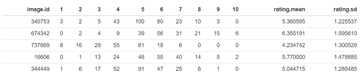
Sample images

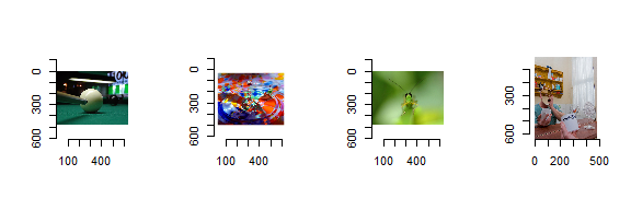Best rated images

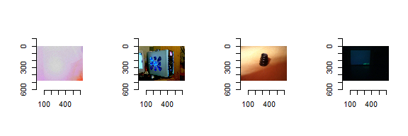Worst rated images

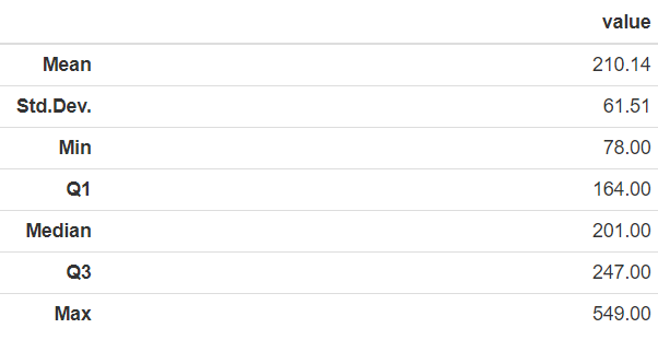
Descriptive Statistics of the number of ratings

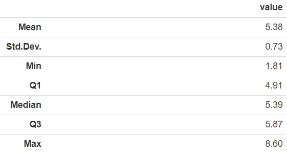
Descriptive Statistics of rating.mean

Exploratory Visualization

Distribution of number of Ratings

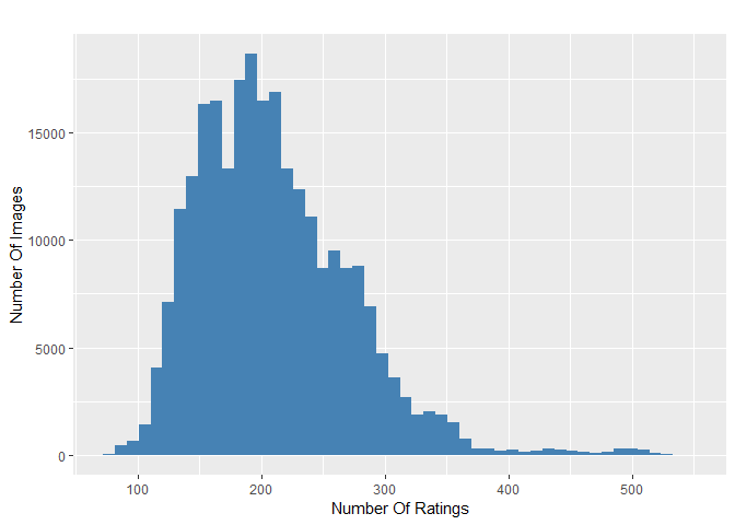
Number of ratings per image: Majority is rated by more than 100 raters

The number of ratings for the images ranges from 78 to 549 with an average of 210 on a scale from 1 to 10.

It can be seen that all images are rated by high numbers of raters. This is very import as rating an image by its aesthetics is very subjective. To level out outliers ratings, a high number of raters is needed.

Distribution of Mean Ratings

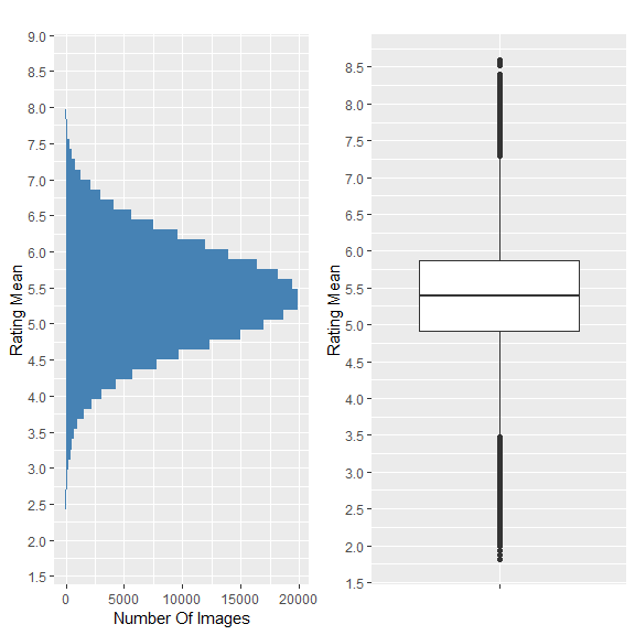
Distribution of rating mean

It can be seen from the distribution and the descriptive statistics that 50% of images have a rating mean within 4.9 and 5.9, and about 85% are between 3.9 and 6.8. From the boxplot, it can be seen that rating means above 7.2 and below 3.5 are outliers in the way that these values are scarce.

This is problematic thas the model performance might not be sufficient for images with excellent and lousy quality.

Algorithms and Techniques

Convolutional Neural Networks (CNN)

A Convolutional Neural Network (CNN) will be used to solve the problem of image aesthetics assessment. They are deep neural networks inspired by biological processes and most commonly applied to analysing visual imagery.

CNN’s consist of an input, an output layer and several hidden layers. The hidden layers are typically a convolutional layer followed by a pooling layer.

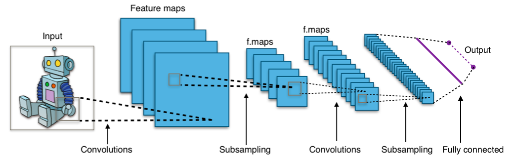
Structure of a typical CNN for image classification. The network has multiple filtering kernels for each convolution layer, which extract features. Subsampling or Pooling layers are used for information reduction. (Source Wikipedia)

Convolutional Layer

The purpose of the convolutional layer is to extract features from the input image. They preserve the spatial relationship between pixels by learning image features using small squares of input data.

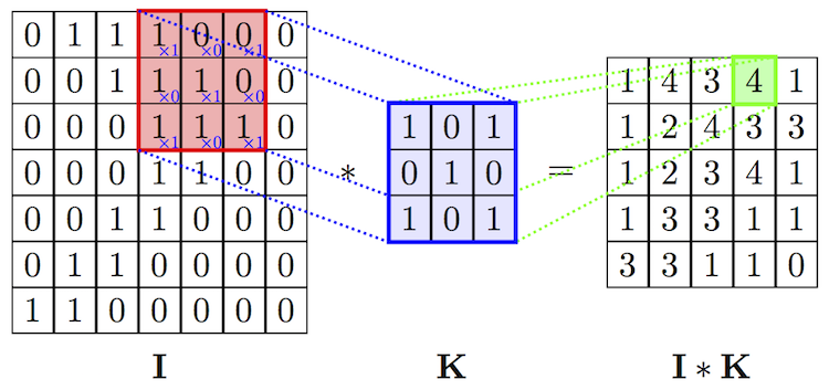
Convolutional operation to extract features

Pooling Layer

Convolutional networks may include pooling layers. These layers combine the outputs of neuron clusters at one layer into a single neuron in the next layer. This is done for the following reasons:

• Reduction of memory and increase in execution speed
• Reduction of overfitting

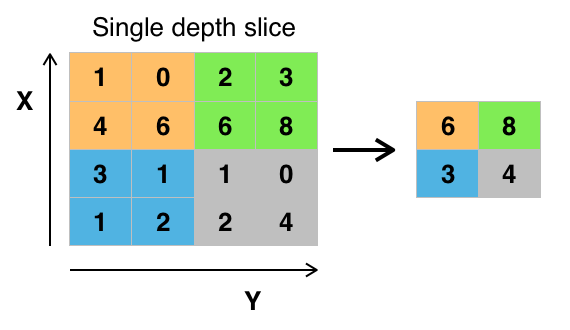
MaxPooling layer, that extracts the maximum value in a region to reduce information. (Source Wikipedia)

Fully connected Layer

After multiple layers of convolutional and pooling layers, a fully connected layer completes the network. The fully connected layer is a traditional multilayer perceptron responsible for the classification task.

Transfer Learning

Transfer learning is a popular method in computer vision because it allows us to build accurate models in a timesaving way (Rawat and Wang 2017). With transfer learning, instead of starting the learning process from scratch, you start from patterns that have been learned when solving a different problem. This way you leverage previous learnings and avoid starting from scratch.

In computer vision, transfer learning is usually expressed through the use of pre-trained models. A pre-trained model is a model that was trained on a large benchmark dataset to solve a problem similar to the one that we want to solve. Accordingly, due to the computational cost of training such models, it is common practice to import and use models from published literature (e.g. VGG, Inception, MobileNet).

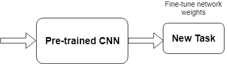
Transfer learning

Several state-of-the-art image classification applications are based on the transfer learning solutions (He et al. 2016), (Szegedy et al. 2016) Google reported in its NIMA (Neural Image Assessment) paper the highest accuracy with a transfer learning-based model (Talebi and Milanfar 2018)

The goal of the project is to use the MobileNet architecture with ImageNet weights, and the replacement of the last dense layer in MobileNet with a dense layer that outputs to 10 classes (scores 1 to 10), which form together with the rating distribution as suggested by (Talebi and Milanfar 2018)

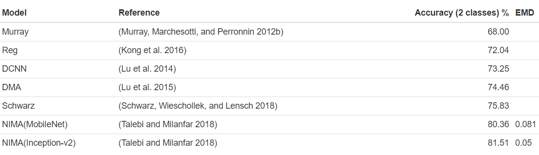
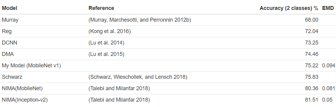
Benchmark

Accuracies of different models on the AVA dataset are reported in different papers. These accuracies are used for benchmarking the models which are created in this project. The benchmarks are based on the “official” AVA test set. The goal is to achieve at least an accuracy of 68% which is above the lower boundary of the relevant papers for image aesthetics.

III. Methodology

Data Preprocessing

The data preprocessing can be divided into two parts: The first part was done during the exploratory data analysis. In this step the following checks and cleanings were performed:

1. Removal of images

   • Several images had to be removed from metadata as they did not exist.
   • Several corrupted images were identified with a script. The corrupted images were deleted from the metadata.

2. Technical image properties were engineered to check image anomalies

   Several technical image properties (file size, resolution, aspect ratio) were engineered and checked for anomalies. No abnormal images could be identified here with these properties.

The second preprocessing step is performed during training:

1. Splitting of the data into training and validation set

   10% of the images of the training set are used for validation.

2. Base model specific preprocessing were performed

   Each base model provided by Keras offers a preprocessing function with specific preprocessing steps for this model. This preprocessing step is applied to an ImageGenerator which loads the images for training and model evaluation.

3. Normalisation of distribution

   The rating distribution was normalised because each image was rated by a different number of people.

4. Image resizing and random cropping

   The training images are rescaled to 256 x 256 px, and afterwards, a randomly performed crop of 224 x 224 px is extracted. This is reported to reduce overfitting issues. (Talebi and Milanfar 2018)

5. Undersampling of the data

   For earlier training sessions the number of images is reduced by cutting the data in 10 rating bins and taking the top n samples of each bin. This is done because of two reasons: As the computing power is limited. This reduces the time to train the model. Another reason is that the data is unbalanced. There are just a few images with very low and high ratings. It was expected that the undersampling reduces the effect of overfitting to the images around the most common ratings.

Implementation

The goal was to create a clear training script which can be parameterised from outside for triggering the different trainings. To reduce the lines of code of this training script, it orchestrates the building blocks of the training with a pipeline script.

1. All needed libraries are identified and put into a requirements.txt

2. An internal library to download the AVA images and the metadata is implemented.

3. A training script was created with building blocks for training (loading data, preparing data, train, evaluate)

4. Building blocks of the training script are moved to a pipeline script. The scripts save different artefacts: Model architecture, model weights, training history, time for training, training visualisation

5. A model class is created, which encapsulates the base model and top model and offers helper functions to change optimiser and freeze layers on the fly

6. The EMD loss function is created

7. The image generator is created for loading the images and perform the preprocessing of the images

8. Several helper functions for model evaluation are implemented

The actual training is performed in 2 Steps:

1. Base model weights are frozen, and just the top model is trained with a higher learning rate

2. Base model weights are unfrozen, and the full network is trained with a lower learning rate

Model design of the CNN

The model consists as mentioned before of two parts. The base model is unchanged apart from the first layers which are removed. The model is initialised with the ImageNet weights. The ImageNet project is an extensive visual database designed for use in visual object recognition software research. The weights for this dataset is used as the images are similar to the ones in the AVA dataset. For the base model, the MobileNet architecture is used as this network is smaller to other networks and suitable for mobile and embedded based vision applications where there is a lack of computing power. (Howard et al. 2017)

The top model consists of two layers. The first layer is a dropout layer to reduce overfitting, followed by a dense layer with an output size of 10 with a softmax activation to predict the distribution of ratings. An Adam optimiser with different learning rates and learning rate decays is used for training.

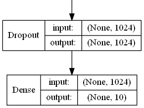
Design of top model: Dropout Layer for avoiding overfitting, Dense layer with 10 output classes

Refinement

Several parameters were used for model refinement:

• Learning rate for dense layers and all layers
• Learning rate decay for dense layers and all layers
• Number of epochs for dense layers and all layers
• Number of images per rating bin used for training
• Dropout ratio for dropout layer in the top model

The training is done iteratively: First, the model is trained with very few samples and the default values for the parameters above. Then the model is trained with more samples, and the parameters are fine-tuned. After the model is trained the loss value and the accuracy are calculated for the test set. The accuracy is then compared against the accuracy scores from the paper (see section Benchmarks) until a sufficient model accuracy was reached.

The training process is supervised with plots for the loss on the training and validation set to check if everything works well and to optimise the learning process.

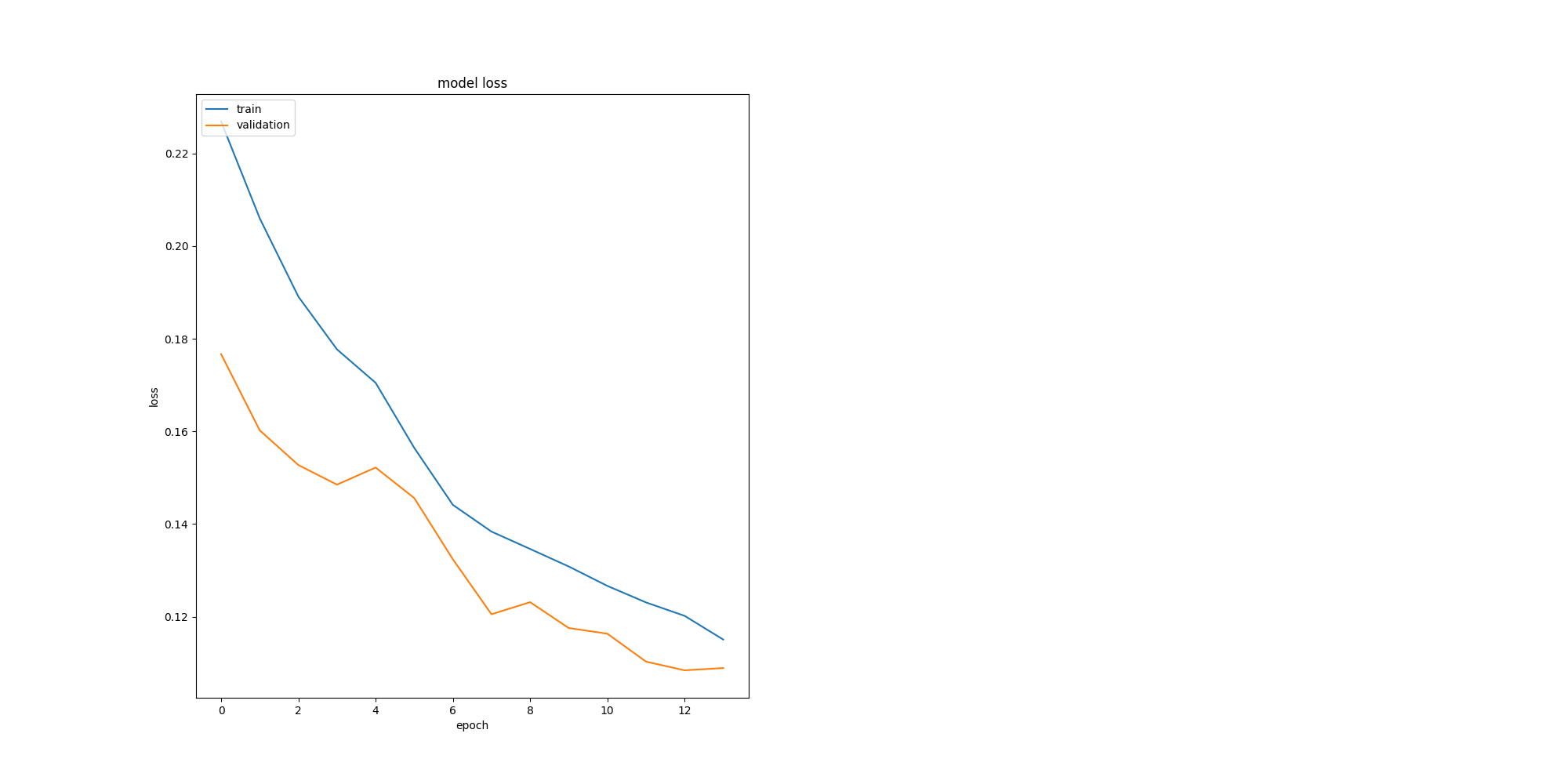
The plots for training history is used to find the best number of epochs for the two learning phases. During phase 1 validation loss flattens at epoch 5 (4 in a plot ) and in phase 2 the val loss flattens at epoch 8 (12 in plot)

IV. Results

Model Evaluation and Validation

Out of the different models model8 was chosen as it’s EMD loss value is the lowest and its accuracy is the highest among all models on the test set. The results are trustful, as the test set is the “official” test set for AVA and the model never saw these images during training or validation. An interesting fact is that this model performs slightly better than model9, which was trained with double the number of training images.

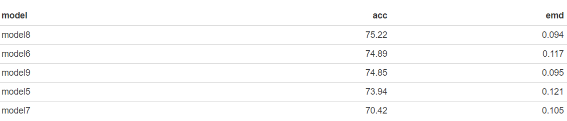
The best model is based on the MobileNet architecture, and the following parameters are used. All these parameters seem reasonable:

It can be seen from the figure below, that the distribution of the ground truth mean ratings and the predicted mean ratings are very similar for the best model. The model works well for mean ratings between 3.5 and 7.5. Ratings below or above these boundaries are not covered well by the model. This due the fact, that there are not many images with very high and low ratings. So the model is not capable of rating these extreme outliers correctly, because of the lack of examples.

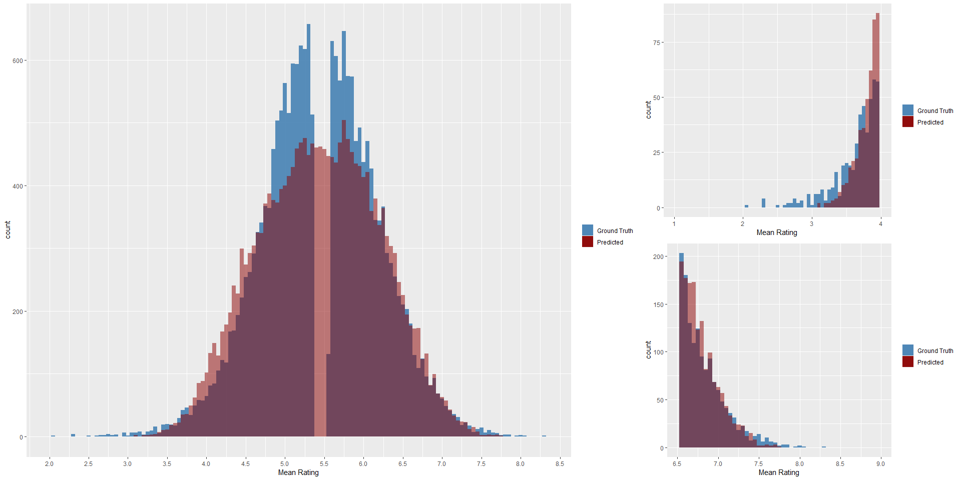
Big figure: Distribution of pedicted mean ratings and ground truth rating on test set. Small figures: Distribution on lower and upper end on test set.

Justification

In comparison to the benchmarks, the model shows a moderate accuracy on the reference test set for AVA which is used throughout all models from the papers.

The result is quite impressive, as the model was trained with just 13914 images. The models in the papers were trained with the full training set.

V. Conclusion

Free-Form Visualization

For a final quick and dirty test the images from the “Project Overview” Section are rated with the model. The images are not part of the AVA dataset.

Left Image: 4.23 Right image: 3.91

Left Image: 3.27 Right image: 4.00

LLeft Image: 3.98 Right image: 4.67

It can be seen, that the images which we as a human being would rate better are also rated better by the model, although the food images are almost the same quality.

Reflection

The process used for this project can be summarised using the following steps

1. A relevant problem was found
2. Research for relevant papers was done
3. Datasets for the problem were researched, analysed and the best a suitable dataset was selected
4. The dataset was cleaned
5. Model benchmarks were extracted from papers
6. The technical infrastructure for the project was set up
7. Models were trained and fine-tuned and checked against the benchmarks, till a good enough model was found, that solves the problem

The project was very challenging for me as I had limited computing power and the dataset is extensive. Till the end, I was not able to train the models on the full training set as there were always problems like running out of memory and Keras and Tensorflow specific problems. I was at some point stuck, as the models poorly performed. After doing an additional research round, I found the Nima paper from Google, which was so brand new that it wasn’t published when I started the project in July. The insights from the paper were a breakthrough, especially a usage of the Earth Movers Loss and the usage of the MobileNet architecture for the base model. I am very proud that I could get an accuracy which was within the boundaries of the relevant papers and mastered a topic that is very hot at the moment, primarily as I used fewer images than the researchers in the papers.

Improvement

It’s exciting that I did achieve an accuracy within the boundaries with my undersampling strategy, which was half born out of need. Even after doing the undersampling of the data the distribution of the ratings is unbalanced.

A strategy to even perform better would be to do image augmentation on the underrepresented rated images. This is not so easy, as not every kind of image augmentation can be used, e.g. darkening an image may affect the aesthetics of the image. Another interesting approach would be to generate images with very high and low rating with GANs (generative-adversarial-networks).

Another improvement for the project would be to containerise the whole process with Docker and Docker NVIDIA. The goal would be to have a docker image that automatically downloads the data, does the preprocessing of it, does the training and stops the container after training. Within this project, this is done with anaconda environments, which is less than ideal in my eyes. I had to always switch from my local environment to the AWS cloud instance, lost time as the environments are not the same. A Docker environment could also be optimised with reusable elements for other Deep Learning projects.

VI. References

He, Kaiming, Xiangyu Zhang, Shaoqing Ren, and Jian Sun. 2016. “Deep Residual Learning for Image Recognition.” In Proceedings of the Ieee Conference on Computer Vision and Pattern Recognition, 770–78.

Hou, Le, Chen-Ping Yu, and Dimitris Samaras. 2016. “Squared Earth Mover’s Distance-Based Loss for Training Deep Neural Networks.” arXiv Preprint arXiv:1611.05916.

Howard, Andrew G, Menglong Zhu, Bo Chen, Dmitry Kalenichenko, Weijun Wang, Tobias Weyand, Marco Andreetto, and Hartwig Adam. 2017. “Mobilenets: Efficient Convolutional Neural Networks for Mobile Vision Applications.” arXiv Preprint arXiv:1704.04861.

Kong, Shu, Xiaohui Shen, Zhe Lin, Radomir Mech, and Charless Fowlkes.

1. “Photo Aesthetics Ranking Network with Attributes and Content Adaptation.” In European Conference on Computer Vision, 662–79. Springer.

Lu, Xin, Zhe Lin, Hailin Jin, Jianchao Yang, and James Z Wang. 2014. “Rapid: Rating Pictorial Aesthetics Using Deep Learning.” In Proceedings of the 22nd Acm International Conference on Multimedia, 457–66. ACM.

Lu, Xin, Zhe Lin, Xiaohui Shen, Radomir Mech, and James Z Wang. 2015. “Deep Multi-Patch Aggregation Network for Image Style, Aesthetics, and Quality Estimation.” In Proceedings of the Ieee International Conference on Computer Vision, 990–98.

Murray, Naila, Luca Marchesotti, and Florent Perronnin. 2012a. “AVA: A Large-Scale Database for Aesthetic Visual Analysis.” https://github.com/mtobeiyf/ava_downloader.

———. 2012b. “AVA: A Large-Scale Database for Aesthetic Visual Analysis.” In Computer Vision and Pattern Recognition (Cvpr), 2012 Ieee Conference on, 2408–15. IEEE.

Rawat, Waseem, and Zenghui Wang. 2017. “Deep Convolutional Neural Networks for Image Classification: A Comprehensive Review.” Neural Computation 29 (9). MIT Press: 2352–2449.

Rubner, Yossi, Carlo Tomasi, and Leonidas J Guibas. 2000. “The Earth Mover’s Distance as a Metric for Image Retrieval.” International Journal of Computer Vision 40 (2). Springer: 99–121.

Schwarz, Katharina, Patrick Wieschollek, and Hendrik PA Lensch. 2018. “Will People Like Your Image? Learning the Aesthetic Space.” In Applications of Computer Vision (Wacv), 2018 Ieee Winter Conference on, 2048–57. IEEE.

Szegedy, Christian, Vincent Vanhoucke, Sergey Ioffe, Jon Shlens, and Zbigniew Wojna. 2016. “Rethinking the Inception Architecture for Computer Vision.” In Proceedings of the Ieee Conference on Computer Vision and Pattern Recognition, 2818–26.

Talebi, Hossein, and Peyman Milanfar. 2018. “Nima: Neural Image Assessment.” IEEE Transactions on Image Processing 27 (8). IEEE: 3998–4011.

Written on March 20th, 2019 by Jens Laufer